Cost function approximations (CFAs)

CFAs have been a hidden secret — widely used in industry (in an ad hoc way), but completely ignored by the academic literature on stochastic optimization.

In a nutshell, CFAs start with a deterministic approximation and then introduce simple parameterizations to make them work well over time. Technically CFAs do not plan into the future (that would be a deterministic direct lookahead approximation), but we are going to handle both of these cases together.

We divide the discussion between problems where $x$ is a discrete action (left/right, color, choice of drug, discretized price), and problems where $x$ is a vector-valued decision.

CFAs are an exceptionally powerful policy in practice. They are discussed in depth in Chapter 13 of Reinforcement Learning and Stochastic Optimization.

Discrete actions

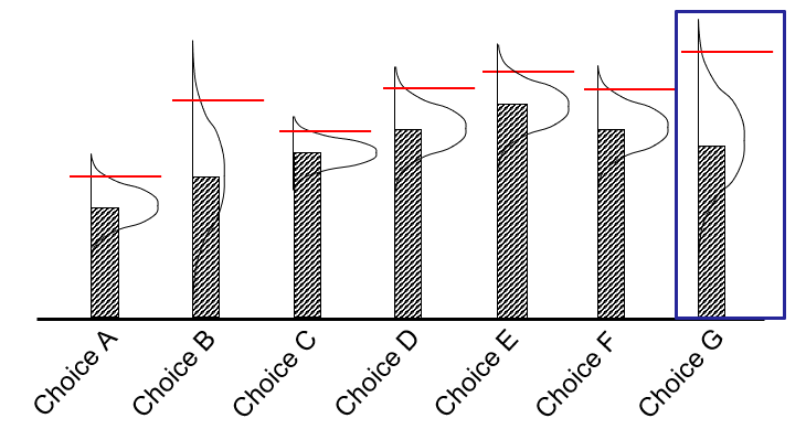
A bar chart of seven discrete choices A–G with hatched bars showing current point estimates, sketched probability distributions, and red horizontal markers showing upper-confidence-bound values; Choice G is highlighted in a blue rectangle as the choice the UCB policy would pick

Imagine you have a set of seven choices as depicted in the figure to the right. You have estimates of the value of each choice — the solid bars — but they are just estimates. The real value is assumed to be somewhere in the probability distribution. If we try a choice, we observe its performance and can use this observation to update the belief. For the vast majority of applications, the beliefs are correlated, which means observing the performance of one allows us to update the estimates of the others.

A simple but highly effective policy known as interval estimation — which falls in a class of policies known as upper confidence bounding — works as follows:

\[X^{IE}(S_t \mid \theta^{IE}) = \arg\max_x \big( \bar\mu_{tx} + \theta^{IE} \bar\sigma_{tx} \big)\]

where $\bar\mu_{tx}$ is our current best estimate of the performance of choice $x$, and $\bar\sigma_{tx}$ is the standard deviation of this estimate. If $\theta^{IE} = 0$, we evaluate each choice based on our current estimate. If $\theta^{IE} = 2$ (say), we evaluate each estimate as if the truth were 2 standard deviations above the point estimate.

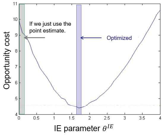
A plot of opportunity cost (vertical axis) versus the IE parameter θ^IE (horizontal axis), showing high cost at θ=0 (the point-estimate case), a clear minimum near θ≈1.7 (the optimized parameter), and rising cost for larger values

First, note that the policy has an “$\arg\max_x(\cdots)$” in it — an optimization problem, albeit a simple one (it requires computing a sort). The challenge is tuning $\theta^{IE}$, and determining whether there is any benefit from using a value other than zero. The answer is an unequivocal yes.

The figure shows the opportunity cost of a policy, where smaller is better. If $\theta^{IE} = 0$ the opportunity cost is much higher than if $\theta^{IE} \approx 1.7$, which performs much better.

Computer scientists have published an extensive literature proving properties such as regret bounds for policies such as this, but they are not optimal policies. However, properly tuned they work well and are widely used — for problems such as deciding the best products to advertise on a web page.

Vector-valued decisions

There are many problems that are traditionally solved using large-scale deterministic optimization solvers. Examples include:

Airlines optimizing schedules with schedule slack to handle weather uncertainty.
Manufacturers using buffer stocks to hedge against production delays and quality problems.
Grid operators scheduling extra generation capacity in case of outages.

In practice, users introduce creatively chosen parameters such as extending the estimated travel times for aircraft to account for weather delays. Grid operators introduce constraints to make sure that power needs will be met even if the largest generator (typically a nuclear plant) fails.

The math-programming community that works with deterministic optimization has turned to a technique called stochastic programming, first introduced by George Dantzig in 1955. It is a difficult, clumsy technique — which explains why real applications appear to be quite rare.

Modifying deterministic optimization models using carefully chosen parameters allows informed users to adjust the model in a way that responds to anticipated uncertainties.

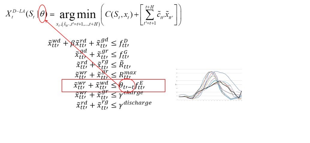
$An illustration of a parameterized deterministic lookahead policy for energy storage: the DLA arg-min formulation shown at top, a system of inequality constraints on storage and wind variables, with a coefficient θ_{t'-t} highlighted on a wind forecast constraint, and a small inset chart showing multiple wind forecast trajectories converging over time$

A simple illustration of a parameterization of a deterministic optimization model is shown above: an energy-storage system being optimized over 24 hours, using point forecasts of wind energy (which is highly uncertain). We multiply the forecast of wind for time $t’$ at time $t$ — written $f^E_{tt’}$ — by a coefficient $\theta_{tt’}$ to account for the uncertainty in the forecast.

Properly tuned, the modified policy performs about 30 percent better than policies where the coefficients $\theta_{tt’}$ are all set equal to 1.0.