Policies

Simply put, policies are methods for making decisions — any method. They can be rules, parametric functions, neural networks, even large-scale integer programs or dynamic programs that depend on Bellman’s equation.

If your decision variable is $x_t$ (always use lowercase for decision variables), the policy would be written $X^\pi(S_t)$ — where $\pi = (f, \theta)$ captures the structure of the function (in “$f$”) and any tunable parameters $\theta$. I often write $X^\pi(S_t \mid \theta)$ to make the dependence on $\theta$ explicit.

If you prefer to use action $a_t$, you would write the policy as $A^\pi(S_t)$, and so on.

Jump to a section

• The four classes of policies
• Hybrids
• Simulating policies
• Evaluating policies
• Optimizing over policies

The four classes of policies

There are two general strategies for creating policies, each of which can be divided into two classes — creating four classes of policies.

Strategy I — Policy search

These strategies create functions that do not explicitly plan into the future to make a decision now. Instead, the functions are designed and tuned to work well over time. They are organized into the first two classes of policies:

1. Policy function approximations (PFAs) — analytical functions that map the information in the state variable $S_t$ directly to a decision to be implemented now. This is the only one of the four classes that does not involve solving an embedded optimization problem.

2. Cost function approximations (CFAs) — deterministic optimization models that are parameterized and tuned to work well over time. CFAs come in two main flavors:

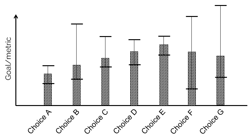
   a. Discrete decisions — $x_t$ might be a choice of drug, a supplier for a part, or a discretized diameter of a wafer. We typically have an estimate of the performance of each choice, but this estimate is not known perfectly. Instead of just picking what appears best, we might use a policy like Upper Confidence Bounding:

   \[X^{UCB}(S_t \mid \theta) = \arg\max_x \big( \text{Est.value}_{tx} + \theta \cdot \text{Std.dev}_{tx} \big)\]

   where:

   • $\text{Est.value}_{tx}$ is the estimated value of alternative $x$ at time $t$,
   • $\text{Std.dev}_{tx}$ is the standard deviation of the estimate,
   • $\theta$ is a tunable parameter: $\theta = 0$ means we just use our current estimate.

   Note the $\arg\max_x$ is an optimization problem, even if it is just a sort over $x$.

   

   b. Vector-valued decisions — $x_t$ might be a vector of decisions assigning machines to tasks at time $t$. These can be large-scale integer programs for scheduling aircraft or manufacturing processes. We can introduce adjustments such as schedule slack, buffers, and other modifications to make the solutions work well over time in the field.

Strategy II — Lookahead approximations

These strategies try to make good decisions now by planning into the future so we can anticipate the downstream effects of decisions made now. Two more classes of policies:

1. Value function approximations (VFAs) — the policies based on Bellman’s equation (the optimal-control community calls these “Hamilton–Jacobi” equations). If you are in state $S_t$ and make decision $x_t$, after which new information $W_{t+1}$ arrives, the net effect is to take you to state $S_{t+1}$ (a random variable when you are making decision $x_t$). If we knew the value $V_{t+1}(S_{t+1})$, we would be able to choose the best decision using Bellman’s equation:

   \[X^{VFA}(S_t) = \arg\max_{x} \big( C(S_t, x_t) + \mathbb{E}\{ V_{t+1}(S_{t+1}) \mid S_t, x_t \} \big)\]

   The problem is that we can virtually never compute $V_{t+1}(S_{t+1})$. Researchers have been trying to develop effective approximations of value functions ever since Bellman in the 1950s — creating fields with names like approximate dynamic programming and reinforcement learning.

2. Direct lookahead approximations (DLAs) — make a decision now by optimizing over a model that spans some time interval (the planning horizon) into the future. We might use a deterministic approximation of the future (very popular) or any of a range of stochastic approximations (such as decision trees).

These four classes of policies span any method for making decisions — including anything in the research literature, any methods used in practice, and even methods that have not been invented yet. That’s why they are called meta-classes.

The first two classes (PFAs and CFAs) are the simplest, along with deterministic DLAs. These three are by far the most widely used in practice. By contrast, VFA-based policies have attracted the most attention from the academic community, followed by stochastic lookahead.

Hybrids

The four classes provide the foundation for a rich array of hybrid policies, such as:

• CFAs with PFAs — choosing the least-cost supplier, but with rules to exclude high-risk companies.
• Lookahead (DLA) with VFA — optimize seasonal production plan, with functions capturing the value of ending inventories.
• Parameterized deterministic lookaheads (DLA / CFA) — plan seasonal production using $\theta$-percentile (say, 80th percentile) demand forecasts.
• VFA policy using PFA — distribution planning using VFAs to value inventory at each warehouse, but using rules (PFAs) to force deliveries to specific locations.
• VFA with CFA — start with a VFA-based policy with a linear model, then tune the parameters of the linear VFA to get the best results using a simulator.

Simulating policies

There are two primary ways of simulating policies:

1. Computer simulations — here we program all the updating equations for the state variable $S_t$ via the state transition model:

   \[S_{t+1} \leftarrow S^M(S_t,\, x_t = X^\pi(S_t),\, W_{t+1}(S_t, x_t))\]

   where we have expressed the possible dependence of new information $W_{t+1}$ on the current state $S_t$ and the decision $x_t$ returned by our chosen policy.

   Computer simulations require capturing the dynamics of the physical system, which can be complex. Often the hardest element is recreating the exogenous information process $W_1, \ldots, W_t, \ldots, W_T$. There are two ways:

   • Sample paths from history. Popular in finance, but requires assuming that $W_{t+1}$ does not depend on current or previous decisions.
   • Sample paths from a mathematical model. For many problems, recreating the properties of the exogenous information process may be the most difficult part of designing a simulator.

2. Field implementations — use a policy in the field and evaluate its performance over time based on actual experience. Watching a process evolve in the field avoids the inevitable approximations of simulators, but it is slow (it takes a week to simulate a week) and requires experimenting in the field, where mistakes can be expensive.

Evaluating policies

With deterministic optimization, we typically have a single objective function (say, total cost) and we are interested in the optimal solution. Evaluating a policy for a sequential decision problem is invariably more complex. In practice, we typically need to pay attention to:

1. Solution quality — on average, plus risk metrics that capture extreme events.
2. Computational performance — average solution times and worst-case behavior.
3. Transparency — how easy is it to understand why a system made a decision?
4. Robustness to data errors.
5. Tuning requirements — are there tunable parameters?
6. Flexibility / adaptability — policies often have to adapt to changing requirements.
7. Complexity / ease of development — is there a risk that a methodology simply will not work?
8. Data requirements.

Optimizing over policies

When we are using deterministic optimization, we want to find the best decision, possibly by solving a problem that looks like:

When we are searching for the best policy, we are searching over functions:

where the system evolves according to

We assume that any constraints are captured in the policy $X^\pi(S_t \mid \theta)$.

The transition from optimizing over decisions $x_t$ to optimizing over policies $X^\pi(S_t \mid \theta)$ is typically a major conceptual hurdle for people coming from a deterministic optimization background. However, this is close to what has been done in statistics and machine learning since linear regression was invented in the 1800s. Imagine we have a dataset $(x^n, y^n)$, for $n = 1, \ldots, N$ observations, where $x^n$ is the input (the “dependent variables”) and $y^n$ are the responses (the “labels”). We want to find a function $f(x \mid \theta)$ that most closely matches the observations $y$ by solving:

In both statistics / machine learning and sequential decisions, the search over functions $f \in \mathcal{F}$ is typically ad hoc. Just as we do with our four classes of policies, the machine learning community picks a class of functions (such as linear models or neural networks), then chooses specific instances within that class, before using the training dataset to do the tuning.