Direct lookahead approximations (DLAs)
I like to describe DLA policies — which explicitly plan into the future — as the policy you use when all else fails. And all else usually fails.
We start by recognizing that we evaluate any policy using the objective function
\[\max_\pi \mathbb{E}_W \Big\{ \sum_{t=0}^T C\big(S_t,\, X_t^\pi(S_t)\big) \,\Big|\, S_0 \Big\}\]where in practice we replace the expectation with simulations of the information process $W_1, \ldots, W_t, \ldots, W_T$. The simulation process is described by our notation:
\[S_0,\, x_0,\, W_1,\, \ldots,\, S_t,\, x_t,\, W_{t+1},\, \ldots,\, S_T,\, x_T.\]Each time we make a decision we can evaluate our performance using $C(S_t, x_t)$, where $x_t = X^\pi(S_t)$. The decision $x_t$ may be a scalar (with discrete or continuous choices), or a vector (possibly high-dimensional) which can again be continuous or discrete. We call this the base model, which can be implemented two ways:
- In a simulator.
- As a mathematical model of the real world.
An optimal policy for this problem is given by:
\[X_t^*(S_t) = \arg\max_{x_t} \Big( C(S_t, x_t) + \mathbb{E}_{W_{t+1}} \Big\{ \max_\pi \Big\{ \mathbb{E}_{W_{t+2}, \ldots, W_T} \sum_{t'=t+1}^T C\big(S_{t'},\, X_{t'}^\pi(S_{t'})\big) \,\Big|\, S_{t+1} \Big\} \,\Big|\, S_t,\, x_t \Big\} \Big)\]This would be nice if we could compute it — but we can’t. In fact, we cannot come close. Instead, we are going to replace the original base model with an approximation that we solve at each time period $t$. This model is called the lookahead model; creating and solving the lookahead model is the basis of DLA policies.
The lookahead model
Since the base model cannot be solved, creating a lookahead model requires replacing it with an approximation that we solve at each point in time $t$ where we need to make a decision. We start by introducing notation for the lookahead model, which parallels the base model:
\[\tilde S_{t0},\, \tilde x_{t0},\, \tilde W_{t1},\, \ldots,\, \tilde S_{tt'},\, \tilde x_{tt'},\, \tilde W_{t,t+1},\, \ldots,\, \tilde S_{tT},\, \tilde x_{tT}.\]The tildes indicate that the state, decision, and information may not be the same as in the base model. All variables are indexed by two time indices: time $t$, which represents the point in time when we are trying to make a decision, and time $t’$, which represents the time within our approximate lookahead model. The base model and lookahead model are illustrated in the figure below.
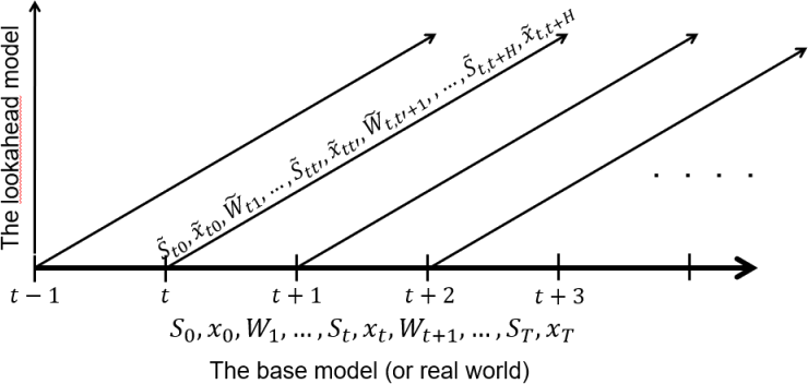
We write our performance metric as $C(\tilde S_{tt’}, \tilde x_{tt’})$, realizing it may have to be modified to accommodate the modified state and decision.
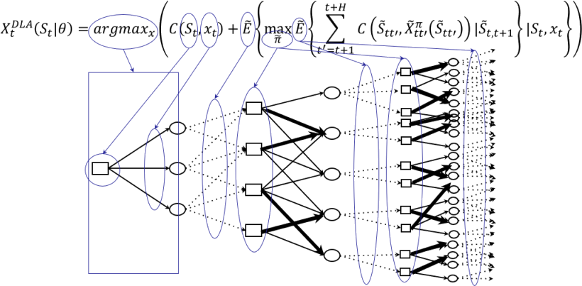
Although we write the decision in the first time period as $\tilde x_{t0}$, when we are done optimizing the lookahead model the first-period decision has to match the decision in the base model — we set $x_t = \tilde x_{t0}$. This notation allows us to write our direct lookahead approximation (DLA) policy as:
\[X_t^{DLA}(S_t) = \arg\max_{x_t} \Big( C(S_t, x_t) + \widetilde{\mathbb{E}}_{\tilde W_{t+1}} \Big\{ \max_{\tilde\pi} \Big\{ \widetilde{\mathbb{E}} \sum_{t'=t+1}^{t+H} C\big(\tilde S_{tt'},\, \tilde X_{t'}^{\tilde\pi}(\tilde S_{tt'})\big) \,\Big|\, \tilde S_{t,t+1} \Big\} \,\Big|\, S_t,\, x_t \Big\} \Big)\]The lookahead policy can be difficult to parse, so it helps to understand what is happening using a decision tree image (below). If $x_t$ is one of a set of discrete actions, then viewing the lookahead as a decision tree can be accurate, although even then we still need to think about the other approximations. We may also view the lookahead as a stochastic simulation, where we determine $x_t$ using the techniques of stochastic search (either derivative-based or derivative-free).
Now the challenge is designing the right approximation that strikes a balance between computational tractability and capturing the important characteristics of the problem as we plan into the future.
Approximating the lookahead model
There are seven categories of approximations that we can apply to our lookahead:
- Deterministic vs. stochastic future — model the future deterministically or stochastically.
- Horizon truncation — while our base model may span time periods $1, \ldots, T$ (which might be quite large), we may feel we can make a good decision by limiting our planning horizon to $t, \ldots, t+H$, where $H$ is the planning horizon.
- Discretization (time, states, decisions) — there are many ways to aggregate the model into coarser representations to simplify computation.
- Latent variables (holding dynamic variables constant) — a latent variable is any variable that may be changing over time in the base model, but which we feel we can hold constant in the lookahead model. For example, we may have rolling forecasts that evolve over time, but we will typically hold a forecast constant within the lookahead model.
- Policy approximation (“policy within a policy”) — for a stochastic lookahead model, we still need to make decisions in the future. We are not going to implement these decisions, but we need to simulate making them many times, so we have to be sensitive to computation.
- Outcome aggregation and sampling — often we will replace a full stochastic process with a small sample so that we reflect an uncertain future.
- Stage aggregation — a “stage” is a sequence of “decision” followed by “information.” Even approximate sequential decision problems can explode if there are enough stages. A popular approximation is to assume that the future is represented as a single stage, where we reveal an outcome over the entire future and then use this outcome to make all decisions.
The first one is the most important choice: are we going to model our lookahead problem deterministically or stochastically? Categories 2, 3, and 4 apply to both deterministic and stochastic lookahead models. Categories 5, 6, and 7 are specific to stochastic lookaheads.
A powerful strategy is to use a deterministic lookahead that is parameterized to make the policy work better under uncertainty. We already covered this under the heading of cost function approximations.