Modeling uncertainty

The literature on sequential decision problems (also known as dynamic programs, reinforcement learning, optimal control, stochastic search, and decision analysis) tends to focus primarily — sometimes exclusively — on making decisions. However, sequential problems are always subject to changing conditions which can be varied and complex.

In most real applications, a good policy for making decisions that works well under realistic conditions (which means accurately capturing uncertainty) is widely preferred over an optimal policy for a problem using a stylized model of uncertainty.

The 12 categories of uncertainty

Chapter 10 of Reinforcement Learning and Stochastic Optimization identifies 12 ways that exogenous information can affect the behavior of a sequential decision problem:

Observational uncertainty — did we detect breast cancer in an X-ray? Do we know the exact location of a driver?
Exogenous uncertainty — covers the wide range of external inputs to a model, including customer demands, equipment failures, weather delays, and human behavior.
Prognostic uncertainty — errors in forecasts of future events.
Inferential uncertainty — errors in estimates of how a market responds to price changes or the condition of a piece of equipment.
Experimental variability — if we run experiments in a lab, a computer simulation, or the field, there is always variability in the results of an experiment.
Model uncertainty — we may not know how disease is being transmitted in a population, or how information about a new product is being spread among consumers.
Transitional uncertainty — a form of exogenous input affecting how the system evolves over time. A classic example is wind buffeting a drone, theft from inventory, or the evolution of the value of an investment.
Implementation errors — arise when decisions from the model are not implemented properly in the field, either from a field operative overriding an instruction (due to local information) or equipment failures (the generator failed to come on).
Communication errors — a different cause of implementation errors, arising from errors in communication, which may come from verbal communication or perhaps international interpretation.
Algorithmic instability — multiple runs of the same algorithm, even for deterministic optimization, can produce different answers for a variety of technical reasons.
Goal uncertainty — different people solving the same problem may produce different answers because they do not share the same goals.
Environmental uncertainty — “environment” spans the entire range from climate, the political climate, the state of the economy, to the emphasis of a management team.

The way to use these 12 categories is as a guide to identifying the forms of uncertainty that might apply to a particular problem. Below, the same checklist is applied to the game of chess, a problem of managing cash for a mutual fund, and a complex public health problem.

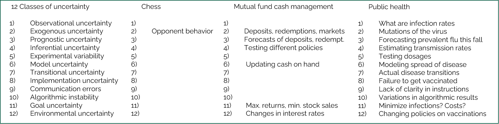
A simple problem such as playing chess would have only one of these, while complex problems such as supply chain management or public health would have one or more sources in all 12 categories.

Modeling uncertainty

There is considerable confusion about how to capture the effect of uncertainty on a sequential decision problem. The biggest problem is that people often focus on how to make decisions. We are going to insist on our “model first, then solve” philosophy — which means we focus first on modeling how the system evolves over time, leaving to later the design of the policy.

Systems evolve from the effect of decisions (that we return to later), and exogenous information that we represent using $W_{t+1}$ after making decision $x_t$ at time $t$. The exogenous information $W_{t+1}$ is best represented as a function:

\[W_{t+1,i}(S_t, x_t) = \text{the information from class } i \in \mathcal{I}^{\inf} \text{ that may depend on the current state } S_t \text{ and/or the decision } x_t.\]

(The classes $i \in \mathcal{I}^{\inf}$ are identified from the framing exercise covered earlier.)

The information $W_{t+1,i}(S_t, x_t)$ may change performance metrics, any of the parameters in our policy $X^\pi(S_t \mid \theta)$, or any other parameters that affect the system in the future (these enter through the state transition model).

Simulating the information process

If we wish to evaluate a policy $X^\pi(S_t \mid \theta)$, we need to be able to simulate the system. We can do this in the field — meaning we simply observe the information processes $W_{t+1,i}(S_t, x_t)$ as they happen, which avoids any need to model the process. The downside is that this is very slow, and we have to live with our mistakes.

The alternative is to create mathematical models that allow us to sample $W_{t+1,i}(S_t, x_t)$. Stochastic models for many systems can be quite subtle and complex. It is tempting to think that all models of uncertainty can be done with normal distributions and Poisson processes (which are popular in textbooks), but those will not take you very far in real-world stochastic models.

The flavors of uncertainty

The evolution of the information processes $W_{t+1,i}(S_t, x_t)$ for the different information classes $i \in \mathcal{I}^{\inf}$ can come in a range of styles, such as:

Hourly / daily variations in demands, prices, etc.
Bursts, spikes, intermittent demands.
Periodic changes from market shifts, competitive behavior, etc.
Regional events (political, regulatory, weather, earthquakes, disease).
Systemic events (cyber attacks, public perception, tariffs).
Black swan events.
Contingencies — events that might happen, but have not happened in the past.
Correlations over time, space, and attributes.

The last item — correlations — is arguably the most difficult and subtle dimension of modeling information processes.