Optimal Learning

The most common sequential decision problems arise when we have two or more choices, typically (but not always) discrete, where we have to make the best choice. The challenge is that we do not know how well each choice will perform, but we can learn from experience to guide future decisions. Examples of these problems are illustrated in the graphic below.

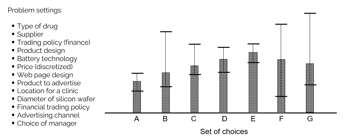
These problems are ubiquitous. We may have two choices, or 10, or thousands. They come in a wide range of problem settings, which we review below. We then review different ways of deciding which choices to try which recognize the value of information on future decisions.

This page is organized as follows:

• Classes of optimal learning problems — the dimensions that distinguish problems: the cost of experiments, offline vs. online, the role of physical resources, and risk.
• The communities of optimal learning — the same problem under many names: bandits, derivative-free stochastic search, Bayesian optimization, design of experiments, ranking and selection, active learning.
• A bit of history — from the 1950s multiarmed bandit problem through Gittins indices to upper confidence bounding (UCB).
• The knowledge gradient for offline learning — a Bayesian, value-of-information policy with no tunable parameters that handles correlated beliefs.
• The knowledge gradient for online learning — a remarkably simple extension of the offline KG.
• UCB policies for offline and online learning — how the same policy can be tuned for either objective.
• KG vs. UCB and the problem of tuning — a direct head-to-head comparison and why tuning is harder than it looks.
• A video application of UCB and KG — a real-world mutual-fund cash-management problem.
• The Knowledge Gradient — the original research — the Test of Time Award paper, the research lineage, and Peter Frazier’s open-source software.

Classes of optimal learning problems

There are countless variations of this basic problem. Two of the most important dimensions are the time and cost for running an experiment (which can range from fractions of a second to months), and whether we are learning in a test environment (a lab or a simulator) or in the field, where we have to live with the results of experiments. Budgets, which may limit the number of experiments that can be run, also play an important role.

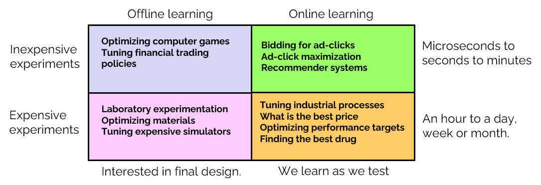
A common thread that runs through all optimal learning problems is known as the “exploration vs. exploitation” tradeoff. This is most prominent when we are learning in the field, since we have to live with poor outcomes. However, the exploration-exploitation tradeoff arises even in offline experimental learning when we are working within a budget.

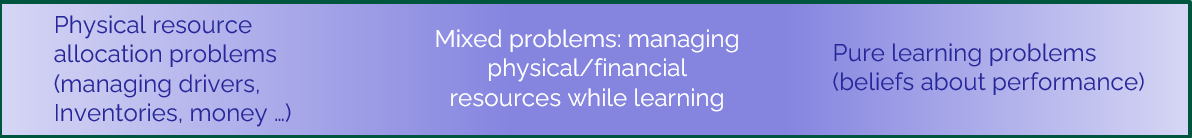
Another important dimension involves the role of physical resources. The classical online learning problem is a pure learning problem where the state of the system consists purely of our beliefs about the performance of each choice. Contrast this with physical resource allocation problems, where the state is given by the quantity of different types and locations of resources. We can create a spectrum of problems that involve a mixture of physical resources and beliefs. The literature that addresses both at the same time is very sparse (check here for examples of problems that combine physical resources with active learning).

Another important element is the consideration of risk. If we are learning in the field, are we willing to accept certain negative outcomes? If we are running experiments in a lab, what is the probability that we are unable to find an acceptable solution within the budget we have set?

The communities of optimal learning

This problem class is so big that it has been studied under a variety of names:

• Multi-armed bandit problems (probability, computer science)
• Derivative-free stochastic search (operations research, applied math)
• Bayesian optimization (probability, applied math, operations research)
• Design of experiments (statistics)
• Ranking and selection (simulation)
• Active learning (machine learning)
• Intelligent trial-and-error (general use)

Each of these terms describes a field that evolved in one community, but they have grown and started to blend. The bandit literature focuses primarily on online learning where experiments are done in the field, whereas stochastic search is typically cast as a problem being solved in a computer in an offline setting. Both communities are solving sequential decision problems that address active learning.

A bit of history

The first research that addressed the “exploration-exploitation” tradeoff emerged in the 1950s under the name “multiarmed bandit problems,” although the first research on derivative-free stochastic search (technically the same problem) appeared in 1951. It was the work on bandit problems that was cast in an online setting where the exploration-exploitation tradeoff is most apparent. The bandit problem was formulated as a dynamic program where the state was the beliefs about the performance of the different choices (“arms” in bandit-speak), but Bellman’s equation was computationally intractable.

The first optimal solution to the bandit problem appeared in 1974 due to John Gittins, who introduced what his former thesis adviser would later name “Gittins indices.” This was viewed as a major breakthrough, since it reduced a $K$-dimensional problem (if there are $K$ arms) to $K$ single-dimensional problems, where Bellman’s equation could be solved numerically.

Although Gittins indices were a computational breakthrough, they were cumbersome to use and were not adopted in practice. However, they served as the inspiration for TJ Lai (from computer science) who, in 1984, recognized the power of index strategies, where a value (index) would be computed for each arm, at which point we would test the arm with the highest index.

An example of an index policy known as “upper confidence bounding” (or UCB) is given by

where:

• $x \in \mathcal{X} = {x_1, x_2, \ldots, x_K}$
• $\overline{\mu}_x^n$ = current estimate of the performance of choice $x$ after $n$ experiments.
• $N_x^n$ = the number of times that we have tested choice $x$ after $n$ experiments.
• $\theta^{UCB}$ = a tunable parameter.

This is just one example of an entire family of so-called “upper confidence bounding” policies which use different methods for creating optimistic estimates of the true value. If $\theta^{UCB} = 0$ then we are just choosing to test the choice that appears to be best on the basis of the current estimate $\overline{\mu}_x^n$.

Computer scientists found that they could prove properties known as “regret bounds” that established limits on how often we would test alternatives other than the best. This work spawned an explosion of papers from authors who thought the goal was to come up with policies with the best regret bound.

A form of UCB policy that we found worked particularly well was introduced in 1993 by Leslie Kaelbling as “interval estimation” and took the form:

where $\overline{\sigma}_x^n$ was the standard deviation of the estimate $\overline{\mu}_x^n$.

A key feature of IE policies is that the parameter $\theta^{IE}$ did not depend on the units of the problem. We could expect $\theta^{IE}$ to fall somewhere in the range $[0, 3]$.

UCB policies all featured a tunable parameter such as $\theta^{UCB}$ or $\theta^{IE}$. If you check the four classes of policies on the Policies page, UCB policies such as these fall under the category of cost function approximations, which always have one or more tunable parameters. Tuning the parameter requires solving a problem of the form:

where

• $W_x^n$ = the observed performance of choice $x^n$ chosen in the $n^{\text{th}}$ experiment.
• $x^n = X^{UCB}(S_t \mid \theta)$ is the choice made to test in the $n^{\text{th}}$ experiment, given the belief state $S^n = (\overline{\mu}_x^n),\, x \in \mathcal{X}$, which is the belief state of all the alternatives.

UCB-style policies have proven very popular in settings such as e-commerce where it is necessary to quickly identify which product to advertise when a customer brings up a webpage. However, they are not well suited to problems with expensive experiments and (invariably) smaller budgets.

The knowledge gradient for offline learning

In 2007 we started publishing papers based on maximizing the value of information that we called the “knowledge gradient,” the name chosen by Peter Frazier, the Ph.D. student who launched this line of research. Peter’s work focused on the “offline” learning problem where you perform a set of experiments (say in a lab or a simulator), and you only care about the performance of the final solution, without regard to the quality of solutions that are tested during the process of experimenting.

The knowledge gradient is a Bayesian method which exploited prior knowledge about a problem. This approach proved to be particularly valuable for problems where experiments were expensive.

Correlated beliefs

A breakthrough enabled by the knowledge gradient was the ability to handle more complex belief models, starting with the idea of correlated beliefs. This arises when one experiment (say, testing a type of medication) allows you to update beliefs about other choices (say medications with similar properties).

For example, if we are given seven types of medications and we administer type G, what we observe may change our belief about how well G performs, and in addition updates our beliefs of some or all of the other choices.

Most problems in practice exhibit correlated beliefs. The choices may be selling different types of clothes, the features on cars, the performance of different investments, the effect of different continuous parameters such as dosages, temperatures and concentrations. Correlated beliefs is what allows us to make a reasonable guess of the best molecular compound from 10,000 choices using 50 experiments.

How it works

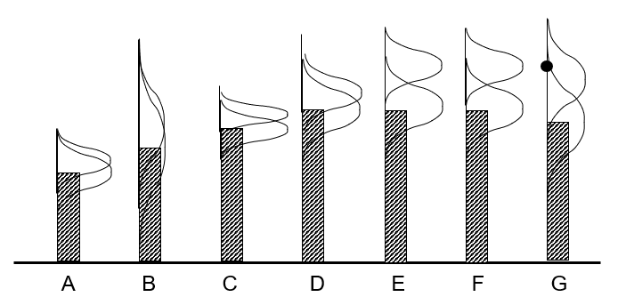
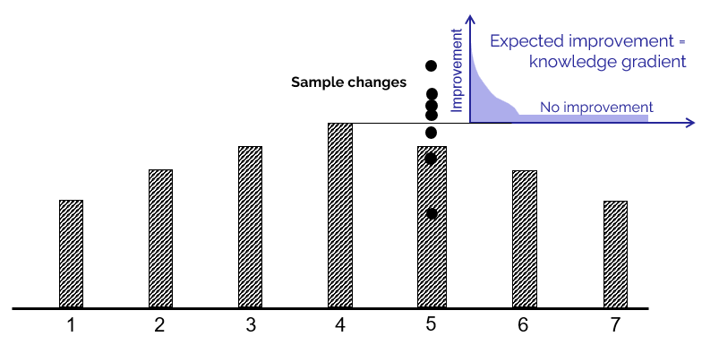The concept of the knowledge gradient is quite simple. Imagine that we have a set of choices where choice 4 seems to be best. However, it is possible that choice 5 is actually best, but has a lower estimate because of errors in initial beliefs or the noise of experiments. If we try experiment 5, we might get any of the results shown as black circles (this is just a small sample). If we obtain any of the lower values and use this to update our belief about 5, we may obtain an updated estimate that is still not as good as choice 4, which means we would not change our decision about which is best.

On the other hand, if we obtain a higher value for choice 5, the result might be that we estimate that 5 is even better than 4. The degree to which the new estimate of 5 exceeds the old estimate of 4 is the value of the information from running an experiment with choice 5. We next build a probability distribution of how much the value improves, which typically produces a spike at zero (no improvement), and a tail of improvements. The mean of this distribution is the expected improvement, which is the knowledge gradient.

Peter Frazier developed a version of the knowledge gradient that captures the effect of correlations, a technique he called the “knowledge gradient for correlated beliefs” (or the “correlated KG” for short). This method won the “Test of Time” award from the journal that published the method. (Click here for more on the correlated KG and the Test of Time award.)

Stated mathematically, the knowledge gradient is given by

where

• $\overline{\mu}_{x’}^{n}$ is the current estimate of the value of choice $x’$ after $n$ experiments, and
• $\overline{\mu}_{x’}^{n+1}(x)$ is the updated value of choice $x’$ after running experiment for choice $x$ (since beliefs are correlated, testing choice $x$ may change our belief about other choices $x’$).

For problems with independent beliefs, the knowledge gradient can be computed with a simple formula that can be implemented in a spreadsheet. For problems with correlated beliefs, we can still compute it exactly, but it requires a simple algorithm.

There is one important feature that the knowledge gradient lacks — it has no tunable parameters. It requires a little more work, but it is much easier to use.

This work served as the basis for six Ph.D. dissertations. For a summary of this work, the Test of Time award, and a link to Peter Frazier’s software library for the knowledge gradient, see The Knowledge Gradient — the original research.

The knowledge gradient for online learning

Transitioning from offline learning to online learning is incredibly easy. Let $\nu_x^{\text{offline},n} = \nu_x^n$ (which we compute above) be the knowledge gradient in an offline setting, which means it only captures the value of an experiment on the final performance of a design. Now let $\nu_x^{\text{online},n}$ be the online version. Assume we have a budget of $N$ experiments which means that after the $n^{\text{th}}$ experiment, we have $(N - n)$ experiments remaining, where we want to maximize the performance of all these remaining experiments. Ilya Ryzhov showed that

This formula captures the natural behavior that if there are many experiments remaining, we want to maximize $\nu_x^{\text{offline},n}$ (since $(N - n)$ is large), while if we have performed only a few experiments, we are going to put more emphasis on doing what appears to be best given what we know by maximizing $\overline{\mu}_x^n$.

UCB policies for offline and online learning

We have just presented two KG policies, one for offline learning and one for online learning. What about UCB policies?

It turns out that you can use the same UCB policy for offline and online learning. The difference is how you tune them. Specifically, what matters is the objective function.

Let $x^{\pi,N}$ be the best “arm” after we have run $N$ experiments using policy $\pi$, where $\pi$ could be any UCB policy (or literally any policy). Assume we are fixing the type of policy (such as the choice of UCB policy), but we are interested in tuning its parameter $\theta^{UCB}$. Let’s evaluate the policy by fixing $x^{\pi,N}(\theta^{UCB})$ — which means fixing the choice $x = x^{\pi,N}$ that we think is best after running $N$ experiments — and run a series of simulations to evaluate it. The results of these “testing” simulations can be written

We then write the problem of optimizing the best choice of $\theta^{UCB}$ as

If we are performing online learning, we would write the performance of the policy as the sum of what we observe, given by

KG vs. UCB and the problem of tuning

The knowledge gradient and UCB policies are best suited for very different problems. UCB policies have proven valuable in high-frequency environments such as identifying the best product to display when a webpage is shown to a user. In that environment, computing the policy has to be hyperfast, and the high frequency of observations makes it very easy to form beliefs.

The knowledge gradient is better for applications where experiments are expensive, which means we need to depend heavily on prior knowledge and carefully developed belief models. We also have plenty of time to perform the calculations needed.

This said, we compared the performance of both policies, focusing on the need to tune the parameter in the UCB policy (we used interval estimation), whereas KG does not need tuning.

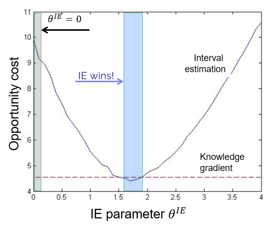
The graph to the right shows the “opportunity cost” curve for the IE policy (where smaller is better). We see that the OC is quite high if $\theta^{IE} = 0$, which means that simply using the point estimate performs poorly. By contrast, KG, which does not have a tunable parameter, works much better.

But KG is not the overall winner! Note that if we can find the best value for $\theta^{IE}$ (around 1.7), IE actually performs better, which is surprising, since this is a problem that exhibits correlated beliefs. KG explicitly handles correlated beliefs, while IE does not. How can this be?

The answer is that we are picking up the behavior of correlated beliefs indirectly from the tuning of $\theta^{IE}$, since we update beliefs using correlations in the simulations. This highlights the power of tuning using a realistic simulator. However, this tuning can be quite hard, since simulating policies tends to be quite noisy.

So, if IE is simpler to use and actually works better, why would we use a more sophisticated (and complex) policy such as KG? First, KG exploits prior knowledge and so is likely to perform much better on very small budgets. Second, we have to emphasize… tuning is hard! Simulating policies is very noisy. The opportunity cost curve in the graphic above is very hard to compute. We obtained this graph by simulating each point 10,000 times, which is simply not possible in practice.

In short, the fact that KG does not have any tunable parameters is a huge advantage.

A video application of UCB and KG

A nice illustration of both a UCB policy (interval estimation) and the knowledge gradient for correlated beliefs is based on a real-world problem of optimizing the amount of cash a mutual fund manager has to keep on hand. This is an example of an online learning problem that we call “Learning while Doing.” The video can be watched here.