SMART-ISO
SMART-ISO is a stochastic, multiscale model of grid operations developed at PENSA (2008–2012), which was designed from the ground up to handle both the variability and uncertainty of growing penetrations of wind and solar. Considerable care was devoted to handling the timing of decisions as well as the ability of PJM’s planning process to adapt as new information becomes available.
SMART-ISO was funded by the SAP Initiative for Energy Systems Research, with considerable support from PJM in terms of data and time spent describing PJM planning processes. The model also benefited from a DOE-funded study, led by the University of Delaware, of high levels of off-shore wind which served as a valuable test of the model.
This summary is organized under the following headings:
- Overview of SMART-ISO
- Calibration — pattern of LMPs, generation patterns
- Study of off-shore wind for the mid-Atlantic region
- Features of the model
- The creation of the “cost function approximation” policy
- Handling uncertainty
- Documentation
Overview of SMART-ISO
 SMART-ISO was intended to be a highly detailed simulator of the PJM power grid, with special care given to the flow of information and the handling of uncertainty. SMART-ISO is much more than a “stochastic unit commitment model” which has received so much attention in the literature and the energy modeling community. It simulates day-ahead and hour-ahead commitment and generation decisions, in addition to real-time economic dispatch at 5-minute intervals.
SMART-ISO was intended as a simulator for performing a wide range of policy studies. It might also be used as a test environment for models and algorithms that might be used in production. It used the full PJM power grid of over 9,000 buses and 14,000 transmission lines in 2010.
A major feature of SMART-ISO was the correct handling of different forms of uncertainty, in addition to the careful modeling of the dynamics of generators such as steam and gas turbines. We paid special attention to the difference between when we make a decision (which determines the information available) and the actionable time (when the decision would be implemented). We carefully distinguished between decisions in the future that will be implemented (e.g. day-ahead decisions on steam generation) and decisions that we use purely for planning purposes (such as day-ahead plans of natural gas combustion turbines).
Calibration
We invested considerable effort into calibrating SMART-ISO against historical statistics from PJM. We used two forms of calibration: matching the pattern of “locational marginal prices” (known as LMPs), and matching generation across different sources. LMPs are the marginal value of supplies at each node, computed using the dual variables returned by the linear program used to model power flows. Accurate LMPs require that loads and grid congestion be accurate over the entire grid.
Pattern of LMPs
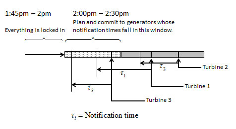 The model carefully captures how PJM handles the “hour-ahead” planning process. The logic, shown to the right, closely matches the PJM IT-SCED logic. IT-SCED is run 15 minutes before and after the hour. The 1:15 run, for example, models the system from 1:30 to 3:30. We look at when each generator is planned to be turned on in this interval, and subtract off the notification time (plus ramp-up time). If this time falls within the interval 1:30 to 2:00, the generator is turned on.
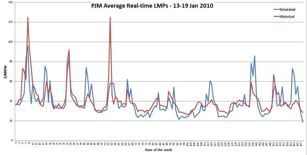
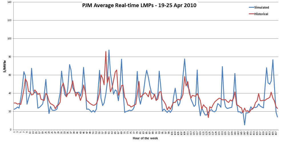
When we introduced this logic, we found that it more accurately reproduced historical LMPs. In particular, look at the latest results for July, and compare to the previous results for July.
Actual vs. simulated LMPs using the new logic that closely matches PJM’s IT-SCED process:
Generation patterns
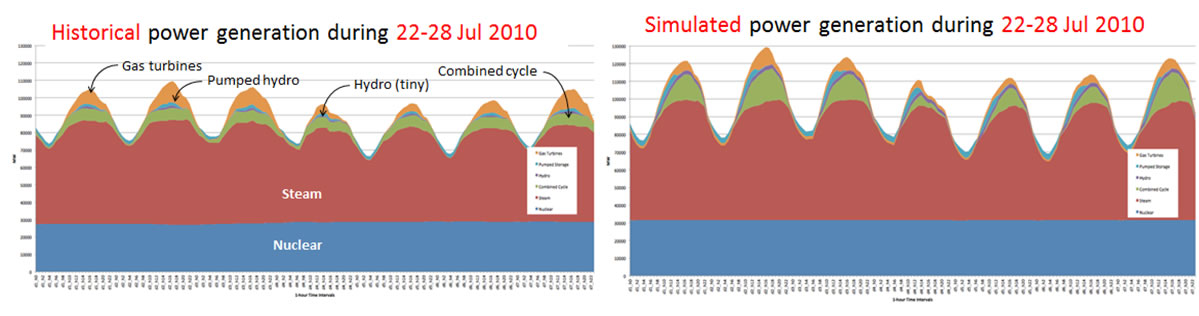
Our first comparison is the distribution of generation across different types of generators, including gas turbines, pumped hydro, a tiny amount of hydro, combined cycle, steam and nuclear. On the left is the historical behavior, derived from the actual generation from PJM but restricted to the generators which we are able to map to the grid (about 93 percent of the total).
On the right is the distribution of generation from the model, where we are running enough generation to cover the entire (actual) load. The plot on the left is slightly lower because we were not able to map all of the generators to the grid.
Note the pattern of pumped hydro, which is charged at night (the bit of blue at night). SMART-ISO initially plans the pumped hydro using a 48-hour look-ahead model, but the actual pumped hydro comes from the hour-ahead model, which required the use of approximate dynamic programming to capture the value of water in the reservoir (without this, the model would simply use all the water right away, rather than waiting until the peak period). The simulated activities are those produced by the economic dispatch model that is run every five minutes.
Study of off-shore wind for the mid-Atlantic region
We performed a careful study of off-shore wind integration with Willett Kempton and Cristina Archer at the University of Delaware (funded by DOE through the University of Delaware). Hundreds of simulations were conducted to design robust policies, and test the limits of offshore wind. Features of the study include:
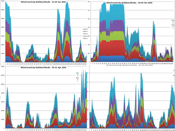
- Five buildout levels were designed, ranging from 8 to 78 GW of capacity.
- We used the accuracy of on-shore forecasts, provided by PJM, to build a stochastic model of the errors in a wind forecast.
- WRF, a popular meteorological model, was used to produce weather simulations for the offshore region, using realistic rolling 48-hour simulations. We created weather patterns for three weeks in each of four months, including January, April, July and October. The stochastic error model was then used to create 7 sample paths for each simulated week, creating 84 sample paths altogether. The WRF simulations for each buildout level, for each month, are shown below.
- Hundreds of simulations of SMART-ISO were run, first to determine the reserves needed to deal with uncertainty. We found the minimum reserve level for each of the four months, for each buildout level.
- Given the reserve levels, we then simulated all 84 sample paths for each of the five buildout levels. We found that we could cover the entire load, for each of the 84 sample paths, for all buildout levels, for January, April and October. Using existing generator fleets, we encountered outages in roughly 20 percent of the scenarios for buildout levels 4 and 5, for the month of July only. This means that we could cover the entire load, for all scenarios, for all months, up to buildout level 3 (40 GW).
Papers describing the offshore wind study:
- Part I: Methodology for forecasting offshore wind
- Part II: Description of SMART-ISO, and results of the offshore wind study
Features of the model
- We used the full PJM power grid, with 10,000 buses and 14,000 transmission lines, but this network can be aggregated upward using a simple parameter setting. If we run the network at, say, a 220 kV level, algorithms are used to map transformers on 69 kV lines to the nearest 235 kV transformers.
- Day-ahead unit commitment — this is an integer programming model which used tunable parameters for spinning reserve and wind to produce a robust solution that can be tuned the next day using the hour-ahead and real-time economic dispatch models. This model uses the DC approximation of power flow within the integer program to produce solutions that are transmission-feasible. Initial experimentation has been conducted to tune the parameters to produce the best robust solution.
- Hour-ahead generation planning — the hour-ahead model assumed a perfect forecast of wind (as of this writing). It fixes day-ahead decisions for nuclear as well as coal and natural gas steam generators. It is allowed to plan natural gas combustion turbine generators in five-minute increments, as well as the use of spinning reserve.
- Locational marginal prices — currently we are producing only day-ahead LMPs. These are coming in at about the right level, but lack the volatility of real LMPs.
- Real-time economic dispatch — we intend to implement a linear programming model to make last-minute adjustments to anticipate actual (vs. forecasted) loads, energy from wind (and solar), generator failures and other adjustments to the grid. When we implement real-time economic dispatch, the hour-ahead model will be switched from using actuals to forecasts of wind, loads, etc.
- Real-time LMPs — we anticipate generating real-time LMPs when we implement the real-time economic dispatch model. Our goal is to try to match the volatility of actual LMPs. To do this, we are planning on introducing different forms of noise into loads, generation and possibly transmission.
- Accurate modeling of off-shore wind — we anticipate having an accurate stochastic model of the errors from forecasting wind, capturing both amplitude (quantity) and temporal errors that arise from meteorological models such as WRF.
- Robust day-ahead policies — we are working on quantile optimization for producing robust solutions from the day-ahead model. This strategy still involves solving a modified (deterministic) integer program, but we anticipate that it will produce lower-cost solutions when we simulate real-time operations the next day.
The creation of the “cost function approximation” policy
It was while working to calibrate the unit commitment model that we realized that PJM (and the other ISOs) were using a very powerful strategy to handle uncertainty. At the time we were developing the model, there were a number of groups implementing a technique first developed by Dantzig (in 1955) called “stochastic programming” which would make a decision “now” (planning the steam generators for tomorrow), while representing the random outcomes tomorrow as “scenarios” which represented samples of different outcomes.
What PJM and the other ISOs were doing was using a deterministic approximation that was then parameterized so that the solutions worked well over time. In our work, we tuned these parameters using our simulator, while PJM (at the time) used their experience in the field.
We decided that what the ISOs were doing, using a parameterized version of a deterministic model, was much more powerful than using stochastic “scenarios.” We gave them the name cost function approximation and it is now one of the four classes of policies that we use to make decisions.
Handling uncertainty
A major feature of SMART-ISO is its handling of uncertainty. Considerable attention has been given in the research community to the “stochastic unit commitment problem” where models use a set of scenarios to handle different events that may happen tomorrow (this algorithmic strategy is known as “stochastic programming”). Instead of a single integer program optimized for a single future, stochastic programming models optimize over multiple scenarios, often producing very large-scale integer programming models that need the power of a supercomputer.
SMART-ISO is first and foremost a simulator, which simulates policies for making day-ahead, hour-ahead and real-time decisions. When a decision (such as day-ahead and hour-ahead) affects the future, we have to design a policy to handle the uncertainties in our forecasts. One goal of SMART-ISO will be to develop and compare different classes of policies for working with uncertainty. Stochastic programming is one class of lookahead policy. Since we wish to simulate these policies over many time periods, computational speed matters, and we will be looking for robust policies that are much easier to solve than the stochastic programming algorithms.
Separate from the design of a policy (an algorithmic challenge) is the modeling of uncertainty. If we think of a policy as a black box for making day-ahead, hour-ahead and real-time decisions, we then have to think about how to model both the dynamics of the physical system (e.g. ramp rates), as well as the dynamics of uncertain events such as wind, solar, loads, and network performance.
We put considerable care into the proper modeling of forecasts of exogenous events such as wind, and the need to do advance planning, such as day-ahead planning of steam generation, planning of gas turbines over 5-to-60-minute horizons, in addition to different forms of demand response which might require advance notification of several hours to a few minutes (or nothing at all). For example, we are developing models of forecast error for wind which captures both amplitude (quantity) and temporal errors. Temporal errors arise when we forecast an increase / decrease in wind due to the arrival of a high- or low-pressure zone, but where the timing is wrong.
We modeled the following types of uncertainty:
- Energy from renewables (wind and solar) — a version of this is already running, but more sophisticated models are planned.
- Loads (due to errors in our ability to forecast weather).
- Generator failures.
- Transmission failures.
Documentation
A summary of SMART-ISO (no equations) is given in Hugo P. Simao, W. B. Powell, C. Archer, W. Kempton, “The challenge of integrating offshore wind power in the US electric grid. Part II: Simulation of the PJM market operation.”